This blog was written by myself, Amelia Woodward, and Tracy Cai as part of the Stanford CS224W course project. It was featured as one of the best final projects of the course, and published on the Stanford CS224W Graph ML Tutorials page.

Traffic is everywhere, on roads, highways, rail networks, and in pedestrian zones. The task of predicting future traffic congestion based on historical and live data is highly relevant to everyone — from companies trying to deliver goods on time to individuals just trying to get to the next Dodger’s game. Traditional and machine learning methods that have been historically applied to this problem often fail to capture the spatial relationships inherent in traffic data.

Interpreting traffic in a graph format allows for modeling that captures spatial connections between traffic points. As a result, graph neural networks (GNNs) are being developed and experimented with for the purpose of traffic forecasting. This post explores the use of GNNs for traffic forecasting, and in particular explores the ST-GAT model developed by Zhang et al in “Spatial-Temporal Graph Attention Networks: A Deep Learning Approach for Traffic Forecasting”. We present our open source implementation of the ST-GAT model (there is not a code base publicly available from the authors of the paper), as well as an explanation of the model, data preprocessing tools, and the results.

You can find the full implementation of the ST-GAT model at on Github: 

Furthermore, we provide a colab for ease of exploring the material.

Dataset

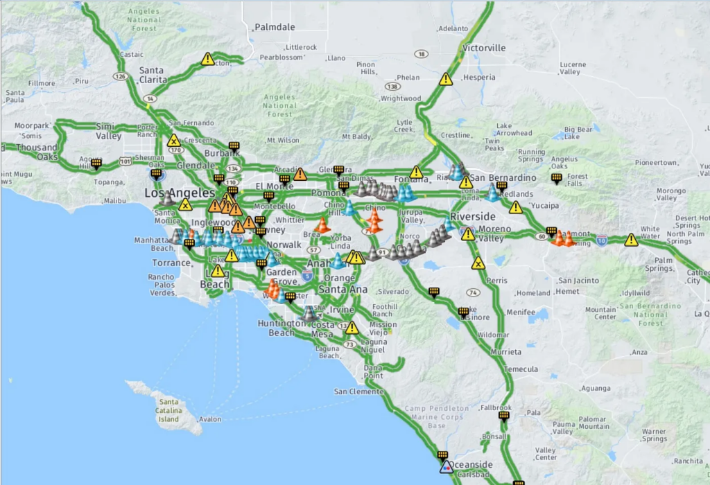
We use the PeMSD7 dataset provided by the Caltrans Performance Measurement System which has more than 39,000 sensor stations collecting real time data across California [3]. The PeMSD7 dataset consists of real-time speed records collected by 228 sensor stations in California District 7 from May 1st to June 30th 2012 (the map below shows the sensor location in the seventh district, mainly covering Los Angeles area). These speed records are then aggregated every 5 minutes.

Pre-processing: Traffic Data into Traffic Graphs

We transform the unprocessed dataset into a dataset of graphs for the purpose of representation and training. Specifically, for each aggregated time point t, we construct a graph

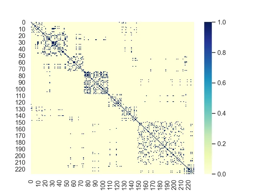
where V is a set of traffic measurement nodes. Each node feature v_t is the average velocity of traffic as measured at the node at time t. In our dataset there are 228 nodes each representing a sensor location in the LA traffic measurement system. E is the set of edges connecting the nodes in V and W is the adjacency matrix. We connect each node based on the distance between traffic measurement sensors. A 1 is used if the nodes are more than a certain threshold distance away, a 0 is used otherwise. A self loop is also added for every node.

Finally, for every timepoint, we construct a dataset object containing all the nodes and their traffic measurements at that time.

The ST-GAT Model

We consider the ST-GAT model for forecasting the average speed of traffic in a traffic network as presented by Zhang et al.

Task Definition

Specifically, at any node and given average traffic velocities at F distinct consecutive intervals, we wish to predict the average traffic velocity in the next H total intervals.

Here F refers to the number of past time steps that are being sequentially considered and H refers to the number of future timestamps. Then we can generalize the prediction task across all sensor stations in the dataset (i.e. all nodes in the graph), to solve the prediction:

This problem is addressed by the ST-GAT model as we describe below, which consists of multiple phases:

1. Data preprocessing: fusing spatial and temporal data using speed2vec

2. An ST-GAT composed of a Graph Attention Network (GAT) and a Recurrent Neural Network (RNN) followed by a fully connected linear layer

Data Preprocessing: Fusing spatial and temporal data using speed2vec

In order to train our Graph Neural Network (GNN), we need to capture both spatial and temporal information. In particular, to add time dependency into the feature vector, instead of simply taking the average velocity at time t as the feature, we will construct a feature h_t that is a vector of F previous measurements. Following Zhang et al [1], we choose to featurize with the velocities from 12 previous time points, so F = 12. We get the featurization:

In the paper, Zhang et al refer to this process of creating a sliding window of features as speed2vec.

TOY EXAMPLE: SPEED2VEC

Here is one quick example to illustrate how the embedding works.

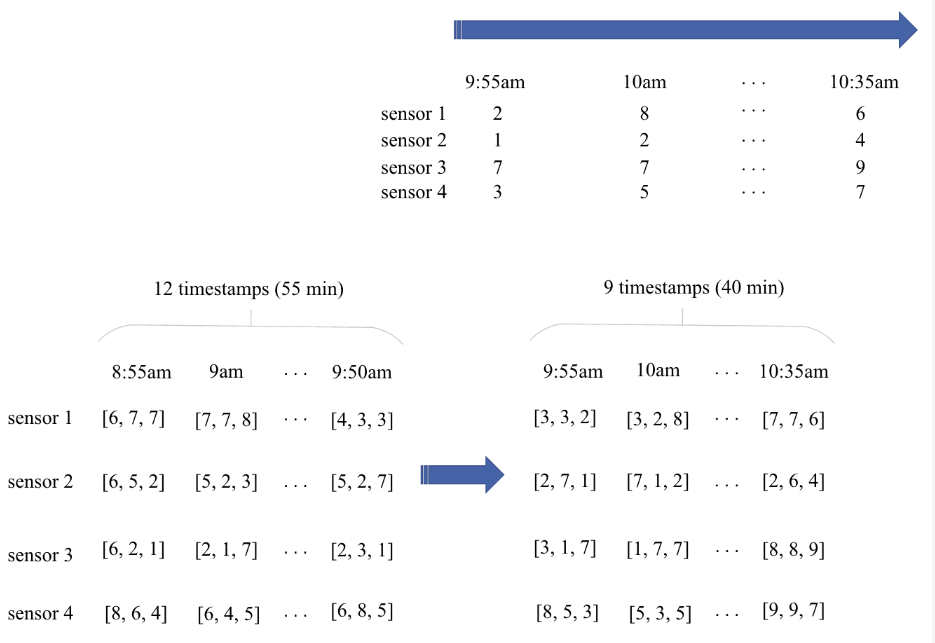
Suppose we have data from four sensors from 8:45 am to 9:10 am. For each sensor v, we have one speed record at each timestamp, given by v_t at time t.

Consider the toy example where we choose F = 3 (feature length 3) and, as described, we have N = 4 (total number of sensors is 4). Suppose that we get sensor readings from data at 5 minute intervals between 8:45am and 9:10am. Then the graph below shows the feature vector we can construct relating to time points 8:55am, 9am, 9:05am and 9:10am, given the information from the previous three time points. We see that we are constructing a sliding window of time features which captures the average velocity of traffic in previous time steps.

Note that since we need the previous velocities from 3 time points, then we cannot fully featurize the first two time points, 8:45am and 8:50am, without information on even earlier time intervals.

Then, by considering all of the nodes in V at time t, we can construct a three dimensional feature matrix across all N nodes AND across all T time points in the dataset, which has dimensions [T, F, N] given by

Here the dimension of length F is not explicitly shown in the above matrix representation.

CODE EXAMPLE: SPEED2VEC

Here is a sample of computing speed2vec-featurized data in our implementation.

In the configuration we calculated the number of slots config[‘N_SLOT’] that can be created in each day’s worth of data (i.e. the number of features of length F=12 that can be produced using a sliding window.

# Access full file at https://github.com/jswang/stgat_traffic_prediction/blob/main/data_loader/dataloader.py
	
sequences = []
# T x F x N
for i in range(self.config['N_DAYS']):
	for j in range(self.config['N_SLOT']):
		# for each time point construct a different graph with data object
                # Docs here: https://pytorch-geometric.readthedocs.io/en/latest/modules/data.html#torch_geometric.data.Data
                g = Data()
                g.__num_nodes__ = n_node

                g.edge_index = edge_index
                g.edge_attr  = edge_attr

                # (F,N) switched to (N,F)
                sta = i * self.config['N_DAY_SLOT'] + j
                end = sta + n_window
                # [21, 228]
                full_window = np.swapaxes(data[sta:end, :], 0, 1)
                g.x = torch.FloatTensor(full_window[:, 0:self.config['N_HIST']])
                g.y = torch.FloatTensor(full_window[:, self.config['N_HIST']::])
                sequences += [g]

We run a sliding window across the velocity data. For each possible consecutive sequence of length F, we construct a speed2vec feature vector with traffic speeds from consecutive time windows. This feature vector is captured in g.x, and the velocities at the next H time steps, captured in g.yform the ground truth for future traffic speed predictions.

We also provide a small tutorial below on using Pytorch Geometric to construct an InMemoryDataset of graph features.

CODE EXAMPLE: CONSTRUCTING A PYG IN-MEMORY DATASET FOR TRAINING

We wrote the following class, TrafficDataset, which is built on the PyGInMemoryDatasetin order to be able to easily feed speed2vec-featurized data into the model.

raw_file_names is a function which returns the path to the raw CSV containing average traffic velocities.

processed_file_namesis a function which returns the path to processed data for the purposes of reloading.

download downloads the files required for the raw dataset.

process actually constructs the TrafficDataset by reading in the raw CSV data, normalizing the data via the z_score method, and for each time point constructing a Data object with a featurization based on the speed2vec processing we previously described. Furthermore, a ground truth prediction is extracted and saved as part of the dataset.

# Access full file at https://github.com/jswang/stgat_traffic_prediction/blob/main/data_loader/dataloader.py

class TrafficDataset(InMemoryDataset):
    """
    Dataset for Graph Neural Networks.
    """
    def __init__(self, config, W, root='', transform=None, pre_transform=None):
        self.config = config
        self.W = W
        super().__init__(root, transform, pre_transform)
        self.data, self.slices, self.n_node, self.mean, self.std_dev = torch.load(self.processed_paths[0])

    @property
    def raw_file_names(self):
        return [os.path.join(self.raw_dir, 'PeMSD7_V_228.csv')]

    @property
    def processed_file_names(self):
        return ['./data.pt']

    def download(self):
        copyfile('./dataset/PeMSD7_V_228.csv', os.path.join(self.raw_dir, 'PeMSD7_V_228.csv'))

    def process(self):
        """
        Process the raw datasets into saved .pt dataset for later use.
        Note that any self.fields here wont exist if loading straight from the .pt file
        """
        # Data Preprocessing and loading
        data = pd.read_csv(self.raw_file_names[0], header=None).values
        # Technically using the validation and test datasets here, but it's fine, would normally get the
        # mean and std_dev from a large dataset
        mean =  np.mean(data)
        std_dev = np.std(data)
        data = z_score(data, np.mean(data), np.std(data))

        _, n_node = data.shape
        n_window = self.config['N_PRED'] + self.config['N_HIST']

        # manipulate nxn matrix into 2xnum_edges
        edge_index = torch.zeros((2, n_node**2), dtype=torch.long)
        # create an edge_attr matrix with our weights  (num_edges x 1) --> our edge features are dim 1
        edge_attr = torch.zeros((n_node**2, 1))
        num_edges = 0
        for i in range(n_node):
            for j in range(n_node):
                if self.W[i, j] != 0.:
                    edge_index[0, num_edges] = i
                    edge_index[1, num_edges] = j
                    edge_attr[num_edges] = self.W[i, j]
                    num_edges += 1
        # using resize_ to just keep the first num_edges entries
        edge_index = edge_index.resize_(2, num_edges)
        edge_attr = edge_attr.resize_(num_edges, 1)

        sequences = []
        # T x F x N
        for i in range(self.config['N_DAYS']):
            for j in range(self.config['N_SLOT']):
                # for each time point construct a different graph with data object
                # Docs here: https://pytorch-geometric.readthedocs.io/en/latest/modules/data.html#torch_geometric.data.Data
                g = Data()
                g.__num_nodes__ = n_node

                g.edge_index = edge_index
                g.edge_attr  = edge_attr

                # (F,N) switched to (N,F)
                sta = i * self.config['N_DAY_SLOT'] + j
                end = sta + n_window
                # [21, 228]
                full_window = np.swapaxes(data[sta:end, :], 0, 1)
                g.x = torch.FloatTensor(full_window[:, 0:self.config['N_HIST']])
                g.y = torch.FloatTensor(full_window[:, self.config['N_HIST']::])
                sequences += [g]

        # Make the actual dataset
        data, slices = self.collate(sequences)
        torch.save((data, slices, n_node, mean, std_dev), self.processed_paths[0])

The Model: Outline and Training

Using our speed2vec-processed training dataset, we are then able to train an ST-GAT model which predicts the average flow of traffic at each node at future time points.

The two major components of the ST-GAT model are a Graph Attention Network (GAT) and a Recurrent Neural Network (RNN). The overall architecture proposed by Zhang et al is included in the figure below.

Graph Attention Network

The first stage of the model is a graph attention network which learns the hidden features with attention information to create new node embeddings. Unlike GCN which uses the sum of features of neighbor nodes for convolution, GAT uses an attention mechanism.

In a traditional GCN model, a message passing algorithm is employed to propagate node features to other connected nodes in the graph.
These messages are aggregated and transformed, and form a new representation of the graph.

In the ST-GAT, the standard Graph Convolutional network is augmented with attention.

An attention mechanism is designed to draw the model’s attention to the most relevant pieces of information in incoming message vectors. Mathematically speaking, this is formulated as: given a set of node features

where N is the number of nodes and F the number of features, we transform the input features into higher level features via a shared weight matrix of some other feature space so that

and a(.) is an attention mechanism function mapping the relationship between the high dimensionally featured input to a score. This score dictates how much the model should focus on the relationship between these two data points.

Upon obtaining attention coefficients, Zhang et al and apply both a softmax function (to normalize the attention coefficients), and a Leaky Rectified Linear Unit (Leaky ReLU) activation function. So the final normalized attention coefficient obtained is

Putting this all together, we see that the ST-GAT updates a node’s internal representation using the following:

The GAT’s message passing and attention are illustrated in the following diagram coming directly from the Zhang et al paper.

Now, to increase the expressivity of attention, Zhang et al actually employ a multi-headed attention mechanism. What this means is that they apply K independent attention mechanisms. In the case of the paper and our implementation, K = 8. Intuitively, multi-headed attention allows the model to learn that multiple different features of the model could be really important, rather than giving the model just a single chance to learn ‘what is important’.

Mathematically, we perform K different sets of the GAT convolution mechanism, one for each of the K heads. Then in order to take these all into account, one can either concatenate all the output features together, or take the mean. These options are illustrated below. In this implementation, we take the average over all attention heads.

GAT Implementation

In our implementation, we use Pytorch Geometric’s GATConv model to perform the attention based message passing described above.

# Access full file at https://github.com/jswang/stgat_traffic_prediction/blob/main/models/st_gat.py
# single graph attentional layer with 8 attention heads
self.gat = GATConv(in_channels=in_channels, out_channels=in_channels,
            heads=heads, dropout=0, concat=False)

in_channels is given by N x T (i.e. the number of nodes in the graph * the number of traffic graphs in the batch;

out_channels is specified in the Zhang et al paper to be 32. We also employ dropout and choose to use averaging to combine the multi-head attention results.

Recurrent Neural Network for Learning Temporal Features

Having learned spatial information about the data using the GAT model, we now feed the output of the GAT into an RNN. The RNN learns temporal aspects of the data for future predictions.

Recurrent Neural Networks (RNNs) are a type of neural network which use outputs from the previous layer as inputs into the next layer and also have hidden states. They are often used for time-series predictions. Zhang et al use Long Short-Term Memory units (LSTMs), which are a practical and highly used variant of RNNs. LSTMs use a collection of gating units and cell states to control the flow of information and solve any issues encountered with the vanishing gradient problem.

An LSTM contains three types of gating units, which for some datapoint at time t has: input gate i_t, forget gate f_t, and an output gate, o_t. Together these three gates decide whether to add or remove information to a cell state.

Given datapoint x_t (which at this point is multi-time transformed feature vector of h_t for some node v at time t), the cell output c_t and the hidden layer output h_t, with relevant weight matrices of the form W_xx and bias vectors of the form b_xx, we can compute the following:

The ST-GAT model uses two LSTM layers and a fully connected linear layer in order to train over temporal sequences. The following diagram shows how the ST-GAT model connects the RNN block and spatial block for a single input feature vector

Note that the blue input blocks correspond to an entire graph’s worth of speed measurements at a single point in time.

Following Zhang et al’s implementation, we use PyTorch’s LSTM layer to create two LSTM layers. The first has a hidden size of 32 and the second has a hidden layer size of 128.

# Access full file at https://github.com/jswang/stgat_traffic_prediction/blob/main/models/st_gat.py
self.lstm1 = torch.nn.LSTM(input_size=self.n_nodes, hidden_size=lstm1_hidden_size, num_layers=1
self.lstm2 = torch.nn.LSTM(input_size=lstm1_hidden_size, hidden_size=lstm2_hidden_size, num_layers=1)

Finally, we apply a fully connected linear layer on the RNN output to extract predictions for the next H time points, where for us, H=9.

For further clarity, we provide a diagram of the training data as it passes from GAT output, through the RNN portion of the ST-GAT and through a linear layer.

The dimensions in the figure below are F=12, N=228 and batch_size=50.

To put the dimensions in context, we are predicting the traffic speeds for the next 9*5 = 45 minutes based on the previous 12*5 = 60 minutes. We do this for all 50 traffic graphs in the batch. The prediction tensor is of dimensions [9, 50, 228], since we predict the next H=9 time points from the previous F=12 time points for each node (sensor station) in all 50 traffic graphs in the batch. We can finally reshape for the purposes of prediction into a two dimensional tensor with dimensions given by [batch_size * num_nodes, num prediction time points] = [50 x 288, 9] = [11400, 9].

TOY EXAMPLE

In our toy example from earlier, if we had F=3, we would be attempting to produce the following predictions. (The diagram assumes we also have access to average traffic velocities at 8:45am, 8:50am also).

The Model Implementation

Our model architecture is captured by the ST_GAT class in Python as follows:

# Access full file at https://github.com/jswang/stgat_traffic_prediction/blob/main/models/st_gat.py
class ST_GAT(torch.nn.Module):
    """
    Spatio-Temporal Graph Attention Network as presented in https://ieeexplore.ieee.org/document/8903252
    """
    def __init__(self, in_channels, out_channels, n_nodes, heads=8, dropout=0.0):
        """
        Initialize the ST-GAT model
        :param in_channels Number of input channels
        :param out_channels Number of output channels
        :param n_nodes Number of nodes in the graph
        :param heads Number of attention heads to use in graph
        :param dropout Dropout probability on output of Graph Attention Network
        """
        super(ST_GAT, self).__init__()
        self.n_pred = out_channels
        self.heads = heads
        self.dropout = dropout
        self.n_nodes = n_nodes

        self.n_preds = 9
        lstm1_hidden_size = 32
        lstm2_hidden_size = 128

        # single graph attentional layer with 8 attention heads
        self.gat = GATConv(in_channels=in_channels, out_channels=in_channels,
            heads=heads, dropout=0, concat=False)

        # add two LSTM layers
        self.lstm1 = torch.nn.LSTM(input_size=self.n_nodes, hidden_size=lstm1_hidden_size, num_layers=1)
        for name, param in self.lstm1.named_parameters():
            if 'bias' in name:
                torch.nn.init.constant_(param, 0.0)
            elif 'weight' in name:
                torch.nn.init.xavier_uniform_(param)
        self.lstm2 = torch.nn.LSTM(input_size=lstm1_hidden_size, hidden_size=lstm2_hidden_size, num_layers=1)
        for name, param in self.lstm1.named_parameters():
            if 'bias' in name:
                torch.nn.init.constant_(param, 0.0)
            elif 'weight' in name:
                torch.nn.init.xavier_uniform_(param)

        # fully-connected neural network
        self.linear = torch.nn.Linear(lstm2_hidden_size, self.n_nodes*self.n_pred)
        torch.nn.init.xavier_uniform_(self.linear.weight)

    def forward(self, data, device):
        """
        Forward pass of the ST-GAT model
        :param data Data to make a pass on
        :param device Device to operate on
        """
        x, edge_index = data.x, data.edge_index
        # apply dropout
        if device == 'cpu':
            x = torch.FloatTensor(x)
        else:
            x = torch.cuda.FloatTensor(x)

        # gat layer: output of gat: [11400, 12]
        x = self.gat(x, edge_index)
        x = F.dropout(x, self.dropout, training=self.training)

        # RNN: 2 LSTM
        # [batchsize*n_nodes, seq_length] -> [batch_size, n_nodes, seq_length]
        batch_size = data.num_graphs
        n_node = int(data.num_nodes/batch_size)
        x = torch.reshape(x, (batch_size, n_node, data.num_features))
        # for lstm: x should be (seq_length, batch_size, n_nodes)
        # sequence length = 12, batch_size = 50, n_node = 228
        x = torch.movedim(x, 2, 0)
        # [12, 50, 228] -> [12, 50, 32]
        x, _ = self.lstm1(x)
        # [12, 50, 32] -> [12, 50, 128]
        x, _ = self.lstm2(x)

        # Output contains h_t for each timestep, only the last one has all input's accounted for
        # [12, 50, 128] -> [50, 128]
        x = torch.squeeze(x[-1, :, :])
        # [50, 128] -> [50, 228*9]
        x = self.linear(x)

        # Now reshape into final output
        s = x.shape
        # [50, 228*9] -> [50, 228, 9]
        x = torch.reshape(x, (s[0], self.n_nodes, self.n_pred))
        # [50, 228, 9] ->  [11400, 9]
        x = torch.reshape(x, (s[0]*self.n_nodes, self.n_pred))
        return x

Walking through the code: in theST-GAT initialization we call upon the GATConv class in Pytorch Geometric for the GAT block, and use Pytorch LSTMs for building the RNN stage of the model. Following the paper, we initialize weights using Xavier initilization. In the forward function we run a forward pass through the model, reshaping the input as necessary to fit the following layers. You can see a full analysis of the dimensionality in our in-line comments (see screenshot or the GitHub linked directly).

Training the Model

In order to train the model, we train using mean squared error (MSE) loss, which is also known as L2 Loss. Specifically, we take the final prediction from the predicted feature vector corresponding to the average traffic velocity prediction at time t + H and calculate the loss between predctions and ground truth average velocities at the corresponding time points.

Furthermore, we train on a train / val / test split of 34 / 5 / 5 where 34 is 34 days’ worth of traffic prediction information and 5 is 5 days’ worth of traffic information.

Evaluation and Results

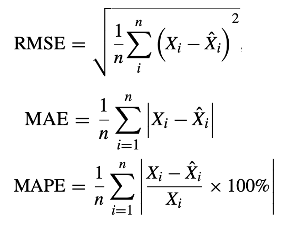
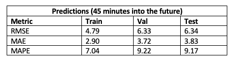
To evaluate the performance of the ST_GAT model, Zhang et al use three different accuracy metrics: mean absolute error (MAE), mean absolute percent error (MAPE), and root mean squared error (RMSE). Their formulas are given below:

In our code implementation, this corresponds to performing the following:

In Zhang et al’s paper, they achieve the following performance when predicting the next 3,6,9 time intervals (which corresponds to 15, 30 and 45 minute periods of time respectively).

Here are the results training our model to predict the next 45 minutes of traffic based on the previous hour of measurements.

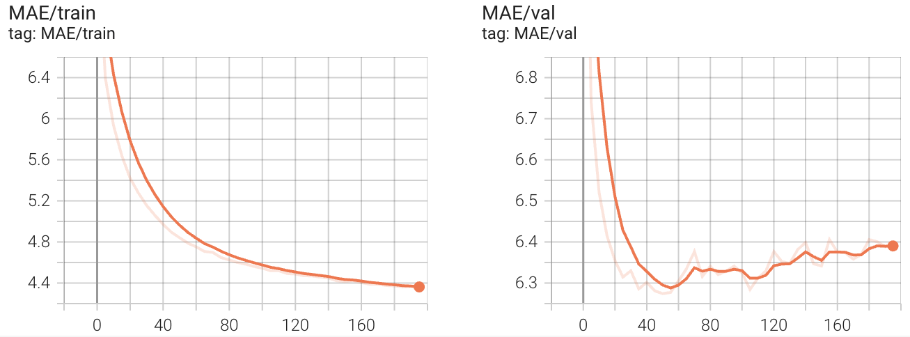
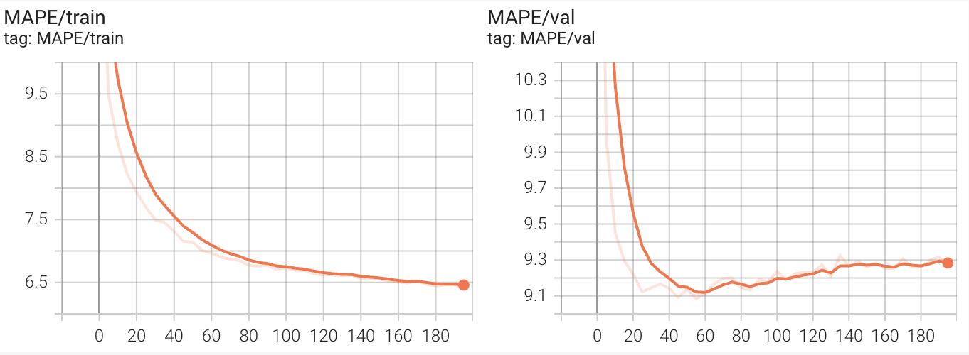
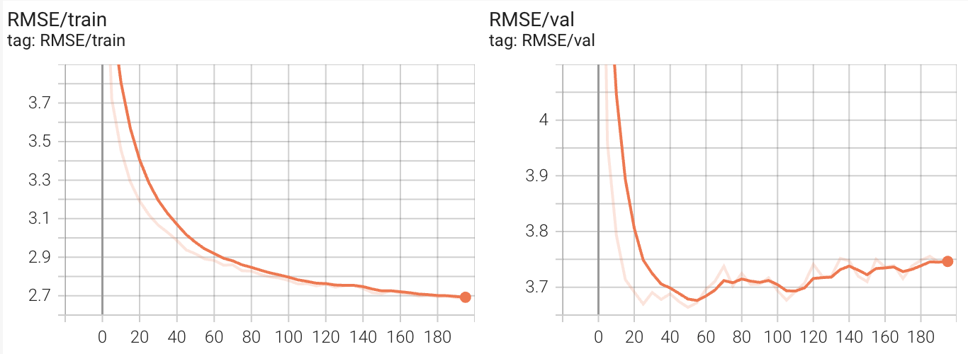
In our implementation, we were able to achieve the following values on the train, validation and test set, getting close to the hyperparameter optimized results given in the paper for the 45 minute time interval.

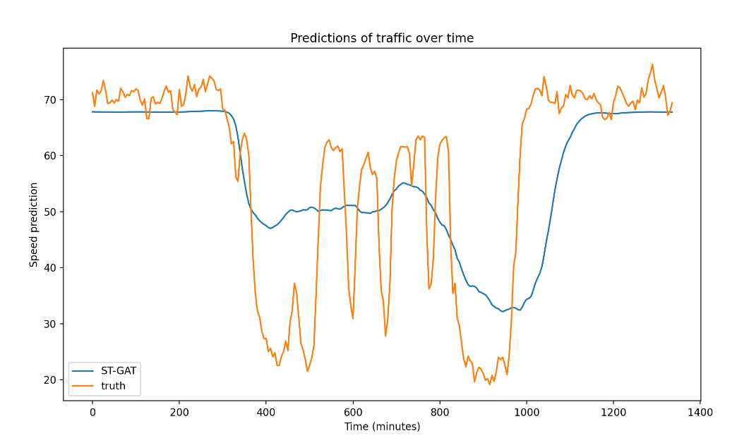
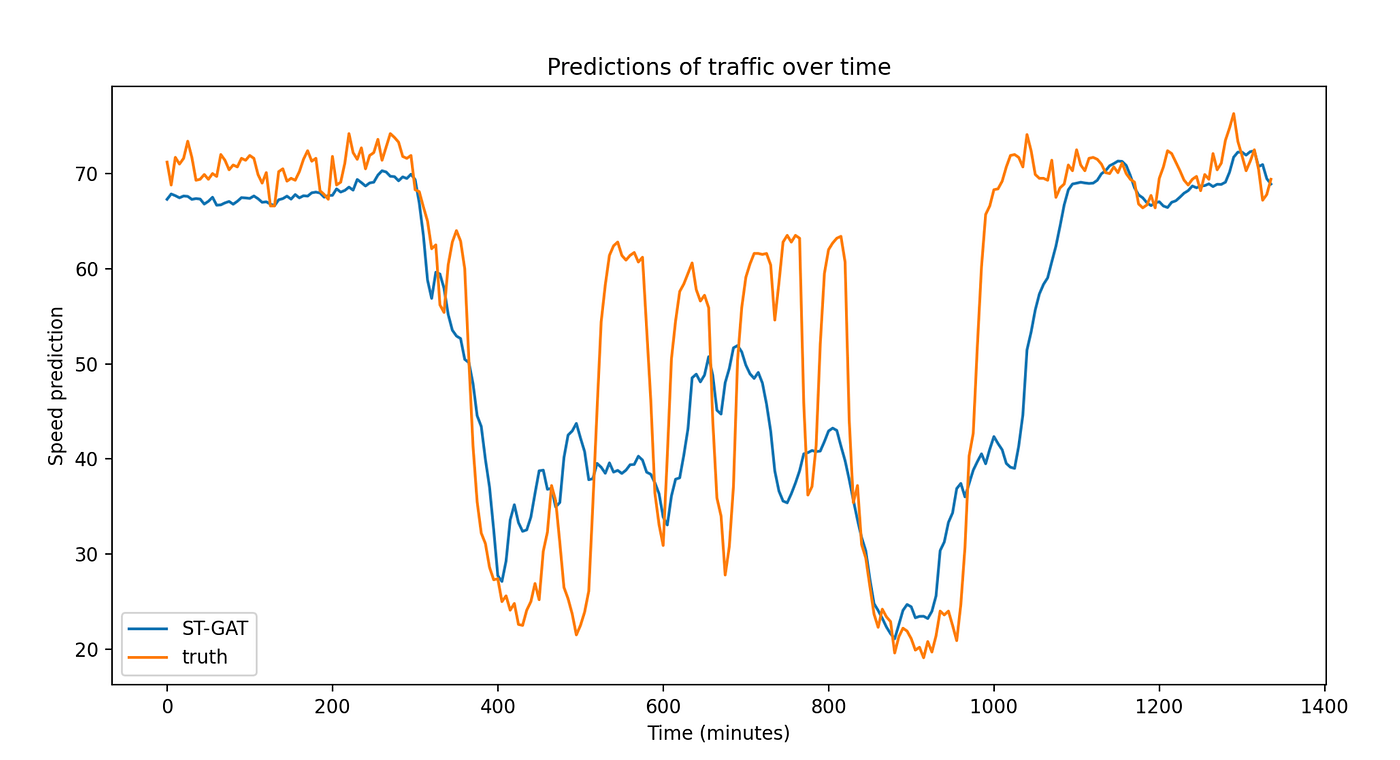
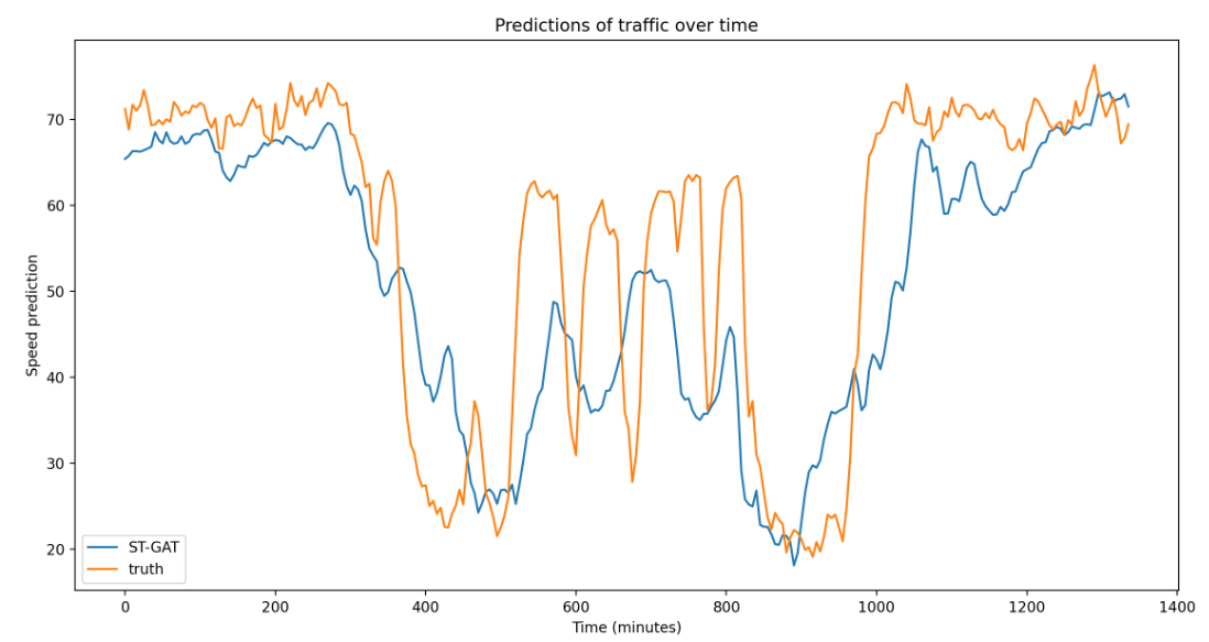
Visualizing predictions

We visualize our resulting predictions after 1 epoch (under fitting), 60 epochs (best predictions) and 200 epochs (over fitting).

Furthermore, we make our implementation of the ST-GAT model available open source on Github. We hope this will be a valuable resource for trying out the GAT model at home, both for traffic prediction and other graph tasks that have both spatial and temporal features.

With additional time and resources, we would be curious to explore a couple of interesting directions of further research. On the data and featurization side, it would be interesting to explore how well the model performs given additional information about road directions, traffic control and weather into the prediction to further improve performance. We would also like to think about even more hyperparameter optimization strategies in order to reduce the overfitting to training dataset. Finally, we would also like to explore the impact of making architectural changes like increasing the number of LSTM layers or trying different attention generating mechanisms emerging in literature.

Find our implementation at: https://github.com/jswang/stgat_traffic_prediction

Find our colab which walks through the code here: https://colab.research.google.com/drive/1NUIQDgj9NXDqtPN_9k_YxKhJN43p3Gho?usp=sharing

References

[1] C. Zhang, J. J. Q. Yu and Y. Liu, “Spatial-Temporal Graph Attention Networks: A Deep Learning Approach for Traffic Forecasting,” in IEEE Access, vol. 7, pp. 166246–166256, 2019, doi: 10.1109/ACCESS.2019.2953888.

[2] Yu, Bing and Yin, Haoteng and Zhu, Zhanxing, “Spatio-Temporal Graph Convolutional Networks: A Deep Learning Framework for Traffic Forecasting”, in Proceedings of the Twenty-Seventh International Joint Conference on Artificial Intelligence, 2018, doi 10.24963/ijcai.2018/505

[3] Performance Measurement System (PeMS) Data Source. Retrieved October 17, 2021, from https://dot.ca.gov/programs/traffic-operations/mpr/pems-source.